
Program Highlights
Undergraduate Program
We offer BA and BS programs that focus on six branches of modern applied mathematics. Undergraduate ProgramApplied Mathematics and Statistics Master’s Program
Our MSE program combines state-of-the-art knowledge with career preparation. Master’s Program in AMSFinancial Mathematics Master’s Program
Our financial mathematics MSE program focuses on quantitative challenges in the global economy and career-readiness. Financial Mathematics master’s programData Science Master’s Program
Our MSE in data science program prepares you for professional advancement and for making an impact on humanity. Data Science Master’s ProgramAMS Doctoral Program
Doctoral students are mentored by renowned scholars and collaborate on research at the frontiers of their disciplines. AMS Doctoral ProgramApply today.
Learn, explore, create knowledge, and make an impact.
Passionate, Creative, Driven, and Inspiring
Get to know us.
Determining Bias in AI - Alexandra Stephens ’19, data scientist at the Johns Hopkins University Applied Physics Laboratory utilizes statistical hypothesis testing to examine whether a performance disparity in AI is due to bias or random chance.
Improving Financial Markets - “The machine learning courses offered at Hopkins helped me establish a wide range of knowledge including the use of models, mathematical principles, algorithms, and optimization skills,” says Yongheng Zhang ’21, a data scientist at Nasdaq’s AI Core Development team.
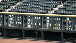
Numbers Game - Alumnus, Neil Gahart, an applied mathematics and statistics major has an abiding love of playing and watching the game. “Being part of baseball’s data-driven present and future has proven irresistible to” says Gahart ’18.
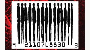
What Are You Worth? - In his book, “Ultimate Price,” AMS alum, statistician, data scientist, and health economist, Howard Friedman MS ’98, PhD ’99 examines all of the ways, hidden and overt, that we affix a finite value to human existence.
-

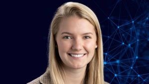
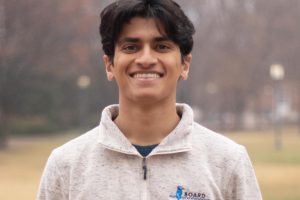
Now leading research at Pink AI, student discovered the power of mathematics as an undergraduate.
-

Making AI Smarter and Greener
CategoriesNew approach could help powerful AI models create realistic content using less energy.
-
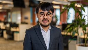
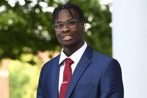
Ishan Kalburge, an applied mathematics and statistic graduate, with a focus on probabilistic deep learning in decision-making, has been awarded the 2024 Gates Cambridge Scholarship.